A History of Molecular Representation
Part 2: The 1960s - Present

James A. Perkins, M.S., M.F.A., CMI
Associate Professor of Medical Illustration
Rochester Institute of Technology


Figure 1. Schematic diagram of a “Richard's box,” a device to construct physical “stick” models of proteins from electron density maps. The user views the density maps through a half-silvered mirror. The mirror simultaneously shows the reflection of the model, allowing the user to align the atoms to the density maps. (Redrawn from Richards, 1968.)

Figure 2. A computer-generated backbone model of lysozyme. The solid tube represents the string of alpha-carbons, amino nitrogens, and carbonyl carbons that runs the length of the amino acid chain. The amino acid side chains are not represented in a backbone model. (©2005 James A. Perkins)

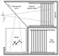
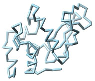
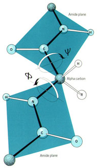
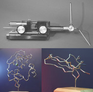
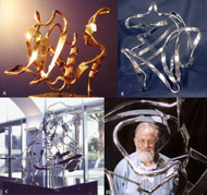
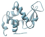
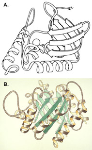
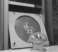
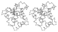
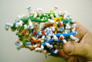
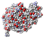
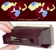
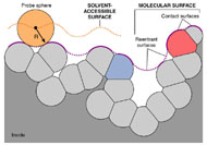
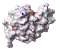
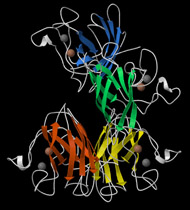
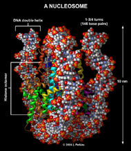
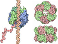
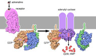
Three-dimensional (3D) Models of Protein Structure

The first installment of this article (JBC 31.1) traced the evolution of molecular representations from the discovery of the atom to the determination of complex macromolecular structures. By the late 1950s and early 1960s, x-ray crystallographers had generated electron density maps of myoglobin, lysozyme, and other macromolecules. This was a painstaking process, involving months of calculations and taxing the earliest computers to their limits. Equally difficult was the process of converting the electron density maps into physical “stick” or Kendrew models. First, the crystallographer constructed a “forest” of vertical steel rods. Each electron density map was held up to the rods and the location of each atom was marked on an adjacent rod by a colored clip. The model was then constructed within the forest of rods, using the clips as a guide. The earliest drawings of a complete protein were made from direct observation of these models (Kendrew, 1961).

In 1968, Fred Richards developed a simpler method of converting electron density maps into 3D models. His optical comparator (Figure 1) used a half-silvered mirror to view the electron density maps while constructing the model, eliminating the need to hold each map up to a forest of rods (Richards, 1968). Known as a “Richard’s Box” or “Fred’s Folly” among crystallographers, this became the standard tool for modeling proteins until the widespread introduction of computer visualization in the 1980s.

One way to further simplify the construction of a protein model is to focus only on the a-carbon “backbone” and ignore the amino acid side chains (Figure 2). The backbone consists of a string of alternating a-carbons, carbonyl carbons, and amino nitrogens that run the length of the peptide chain. The folding of the backbone, and hence the general shape of the protein, is determined by the bond angles between a-carbons and carbonyl carbons (psi bond) and between a-carbons and nitrogens (phi bond) within each amino acid (Figure 3).

One of the most novel approaches to constructing backbone models was “Byron's Bender,” developed by Byron Rubin in the early 1970s (Rubin and Richardson, 1972). By entering torsion and bend angles for every amino acid in the chain, this machine would bend a piece of steel wire into a physical model of the protein backbone (Figure 4). Small, lightweight, and cheap to produce, these models were easy to transport and could be readily compared with one another (Rubin, 1985). This led to further scientific breakthroughs, as illustrated by this story from Eric Martz at the University of Massachusetts, a pioneer in molecular visualization:

An example illustrating the importance of models from Byron’s Bender occurred at a scientific meeting in the mid 1970’s [sic]. At this time, less than two dozen protein structures had been solved. David Davies brought a Bender model of an immunoglobulin Fab fragment, and Jane and David Richardson brought a Bender model of superoxide dismutase. While comparing these physical models at the meeting, they realized that both proteins use a similar fold, despite having only about 9% sequence identity. This incident was the first recognition of the occurrence of what is now recognized as the immunoglobulin superfamily domain in proteins that are apparently unrelated by sequence. (Martz and Francoeur, 2004; see Richardson, et. al., 1976, for the original reference).

Byron Rubin also developed a large-scale version of his “bender,” utilizing a tailpipe bending machine at a local Midas Muffler shop. In addition to his ongoing work as a biochemist, he creates large molecular sculptures at his studio in Rochester, NY. His 5-ft. sculpture of rubredoxin won the Chandler Competition at the University of North Carolina and now resides in the lobby of the Paul Gross Chemistry building at Duke University. A smaller sculpture of human neutrophil collagenase is on permanent display at the Smithsonian (Figure 5; Martz and Francouer, 2004).

Worms and Ribbons

Another approach to visualizing protein structure is to employ a “ribbon” diagram (Figure 6). Similar to a backbone model, a ribbon diagram omits all side chains and makes no attempt to render the surface of the molecule. However, it differs from a backbone model in that bend angles are “smoothed,” producing a model with graceful curves and spirals, rather than the “kinked” appearance of a typical backbone model. More importantly, a ribbon uses graphical symbols to distinguish elements of the protein’s secondary structure, corkscrew spirals for a-helices, flat ribbons for b-strands and sheets, and rounded ‘ropes’ for turns and other non-repetitive structures (Richardson, 2000). The arrowheads on b-strands allow the viewer to trace the peptide chain from its N-terminus to its C-terminus (the direction in which proteins are synthesized from RNA).

Irving Geis was one of the first to use the ribbon metaphor in his book The Structure and Action of Proteins (Dickerson and Geis, 1969a). He used simple spirals to represent the a-helix and flat arrows to show several b-strands forming a sheet. Ribbon drawings appeared sporadically over the next decade (e.g., Holmgren, et al., 1975) and were popularized by Jane Richardson in the 1980s. Richardson originally used her own method of depicting proteins, which she called a “worm” drawing (Richardson, 2000). This was nothing more than a smoothed backbone drawing using a black line of uniform thickness. In 1979, she was asked to do a systematic survey of protein structure for the series Advances in Protein Chemistry. She spent the next year devising a visualization scheme that could capture and classify the structures of all known proteins (75 at the time) and drawing all of them by hand (Figure 7). She borrowed from earlier ribbon diagrams and devised the system that is in use today.

Published in 1981, her survey “The Anatomy and Taxonomy of Protein Structure” established the ribbon diagram as one of the most popular methods of molecular representation. In a recent survey of 103 articles published in the journal Structure, Goodsell (in press) found that “ribbon diagrams are by far the most commonly used representations, for subjects ranging all the way from small hormones to virus capsids. Of the 103 papers, 67 include ribbon diagrams of monomeric and dimeric proteins, and 13 papers include ribbon diagrams of larger oligomers.”

Like other molecular representations, the ribbon diagram is much more than a handy way of publishing structure data. It enabled Richardson to identify the common features of dozens of different proteins and develop a classification scheme for them. One of her drawings even revealed a mistake in the original protein model. She later wrote, “making a drawing can change one’s scientific understanding of a protein" (Richardson, 2000).

Early Computer Models

By processing x-ray diffraction data, computers played a vital role in solving the first structures of macromolecules. As processing power increased over the next few decades, it was only logical that computers would play an increasing role in modeling and visualizing molecular structures.

The earliest computer representations of biological macromolecules were developed by Cyrus Levinthal and his colleagues at MIT in the early 1960s (Figure 8). Using an IBM mainframe and a simple oscilloscope “monitor,” backbone models of simple proteins could be rotated on screen in response to movements of a plastic globe, the predecessor of today’s trackball (Levinthal, 1966). At about the same time, Carroll Johnson at the Oak Ridge National Laboratory developed the Oak Ridge Thermal Ellipsoid Plot Program (ORTEP), a computer program that renders publication-quality stereoscopic drawings of molecules using a pen plotter (Figure 9) (Johnson, 1965). These simple line drawings of backbone models graced the pages of many textbooks throughout the 1960s and 1970s. Currently in its third version, the ORTEP sourcecode and documentation are still available for download from the ORTEP website (www.ornl.gov/sci/ortep/ortep.html).

These early computer programs could not directly interpret electron density data from x-ray crystallographic studies. Instead, the electron density maps were converted by hand into a Kendrew “stick” model which was then measured and its coordinates entered into the computer to construct the virtual model. The next big breakthrough in molecular visualization was the development of computer programs that could convert electron density maps directly into a computer model, eliminating the need to build a physical model. In 1974, the Biographics Laboratory at Texas A&M University used a program call FIT to solve the structure of Staphylococcus nuclease (Collins, et al., 1975). In the late 1970s, T. Alwyn Jones released FRODO, which eventually became the standard tool for building virtual models from electron density maps (Jones, 1978). It is estimated that more than 95 percent of crystallographic structures solved since the early 1980s were built using FRODO or its successor, which is simply called “O” (Jones, 1998).

Molecular visualization software has now come full circle. Instead of measuring a physical model to generate computer coordinates, the virtual model comes first and Rapid Prototyping technology (“3D printing”) can be used to generate a tangible model of the molecule (Figure 10). One such technology aims a laser into a vat of liquid photopolymer, curing the material into a solid. Other technologies build up the model by depositing successive layers of plastic, cornstarch, or other material.

At the Molecular Graphics Laboratory, Scripps Research Institute, tangible models are used in conjunction with computer models to create a sort of “augmented reality” (Gillet, 2005). A tangible molecular model is held in front of a digital video camera. The model appears on a computer screen, turning in real time as the person holding the object manipulates it. Meanwhile, software can superimpose other molecular images that follow the movements of the model. It is a powerful means of demonstrating the interactions between molecules in three dimensions, such as ligands binding to active sites on a receptor protein. For additional information, including a Quicktime® movie demonstrating the process, visit: www.scripps.edu/news/press/032405.html

Molecular Surfaces

While a backbone model simplifies the visualization of protein structure, computers made it possible to show every atom—including the amino acid side chains—and thus determine the external shape of the entire molecule. The development of raster graphics displays made it possible to visualize every atom as a CPK-style sphere (Figure 11), the combination of all spheres producing an image of the protein's surface (Connolly, 1996). In 1980, Richard Feldmann of the NIH used digitally-rendered CPK models to produce Teaching Aids for Macromolecular Structure (TAMS), a set of 116 stereoscopic slides of protein structures, complete with an inexpensive cardboard slide viewer (Figure 12) (Feldmann and Bing, 1980).

A CPK-style model is just one approximation of a protein’s surface. A different, and perhaps more useful, representation is the “solvent-accessible surface” model. In the late 1950s, Kauzmann recognized that hydrophobic amino acid side chains are repelled by water and become buried deep within the protein as the amino acid chain folds (Kauzmann, 1959). Fred Richards and B. K. Lee developed the concept of a solvent-accessible surface to distinguish buried from accessible side chains and to predict the external shape of the molecule (Lee and Richards, 1971). They envisioned a solvent molecule as a sphere of fixed diameter (a “probe” sphere) rolling over the surface of a protein (Figure 13). The probe makes no contact with deeply buried atoms and simply rolls over the van der Waals surfaces of exposed atoms. Adding the radius of the probe sphere to the combined van der Waals radii of all exposed atoms yields the solvent-accessible surface (Figure 14). The probe diameter is typically 1.4 angstroms—the size of a water molecule.

Richards later refined this idea and introduced the “molecular surface” model (Richards, 1977; Richmond and Richards, 1978; reviewed in Connolly, 1996). This model also requires rolling a probe sphere over the surface of a molecule (Figure 13). However, rather than adding the probe radius to the outside of the molecule, the molecular surface consists of the exposed surfaces of the atoms themselves (the “contact surfaces”) plus the concave surfaces between adjacent atoms where the probe cannot reach (the “reentrant surfaces”). Jonathan Greer and Bruce Bush (1978) were the first to develop digital images of a molecular surface while analyzing interfaces between the four subunits in a hemoglobin molecule. Their study demonstrated one of the advantages of the molecular surface model: “..its ability to visualize shape complementarity at interfaces " (Connolly, 1996). The concept of shape complementarity has become extremely important in the pharmaceutical industry—using computer models to match potential drugs to receptors, antibodies, and other proteins. Thus the development of a new type of molecular representation paved the way for a whole new field of scientific inquiry.

The Protein Databank

In the early 1970s, only a handful of macromolecule structures were known. Nevertheless, it was clear that these structures needed to be held in a common repository to facilitate further research. In 1971, the Protein Databank (PDB) was established at the Brookhaven National Laboratory with just two protein structures. A handful of structures were added each year until the 1980s, when the database began to grow exponentially. The introduction of computer software to interpret electron density maps, the development of new crystallographic methods such as NMR spectroscopy, and a greater willingness of academics to share their data all contributed to this growth (Berman, et al., 2000, 2004). Many academic journals and funding agencies also mandated that crystallographic data be deposited in the PDB. As a result, “the current rate of data deposition is about 5,000 structures per year, which is more than double the rate of 5 years ago" (Berman, et al., 2004: 53). In 1998, management of the PDB was transferred to the Research Collaboratory for Structural Bioinformatics (www.rcsb.org/pdb).

The development of the World Wide Web in the 1990s profoundly changed the way PDB data was accessed. Prior to that time, molecular coordinate files were distributed on magnetic media to a small number of researchers in crystallography and structural biology. Now these files can be downloaded in a matter of seconds by researchers in a variety of fields as well as educators and students at all levels. The PDB currently receives more than 160,000 Web hits per day (Berman, et al., 2000). Dozens of additional databases have appeared, archiving specific protein types (e.g., antibodies, membrane proteins), nucleic acids, lipids, drugs, and inorganic compounds. Examples include:

• The Nucleic Acid Database
  
• ChemID-Plus from the National Library of Medicine (125,000 organic and inorganic molecules)
  
• Directory of Antibody Structures

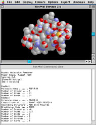
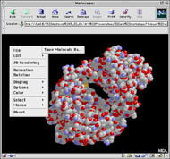
Hundreds of other sites can be found at the World Index of Molecular Visualization Resources.

Desktop MolVis Software and the Internet

As molecular model files became more readily available, so did the software to view and manipulate them. This was further spurred by the availability of inexpensive desktop computer systems. In 1991, Per Kraulis released MolScript (Kraulis, 1991) which enabled researchers to produce their own ribbon diagrams of proteins. Until recently, this was the standard program for producing publication-quality renderings of molecular structures. The following year, David and Jane Richardson released Mage for the Macintosh (Figure 15), a tool for viewing kinemages (“kinetic images”) interactive animated images of molecules (Richardson and Richardson, 1992). This was the first MolVis application designed specifically to run on a desktop computer. It was included on a diskette with the first issue of the journal Protein Science, making it widely available to biologists and chemists.

Perhaps the single most important event in the history of digital molecular visualization was the release of RasMol in 1992 (Figure 16) (Sayle and Bissell, 1992). As an undergraduate, Roger Sayle developed a ray-tracing algorithm that could shade solid objects as they rotated in space. He applied this algorithm to molecular structures and released RasMol (Raster Molecule), first for specialized multiprocessor computers, then for UNIX, and ultimately for Macintosh and Windows. Upon receiving his doctorate, Sayle released RasMol and its C language sourcecode on the Internet (Sayle and Milner-White, 1995). This made it available to a huge audience that otherwise would not have access to MolVis software. It is estimated that more than one million people still use the program (Martz and Francoeur, 2004).

The RasMol sourcecode also has been incorporated into dozens of other MolVis applications. For example, Molecular Simulations, Inc. (MSI) developed WebLab ViewerLite and WebLab ViewerPro, two standalone applications based on RasMol. The free “Lite” version has become very popular with illustrators as it allows export of VRML files that can be imported into 3D modeling applications for high-quality rendering.

In 1996, MDL Information Systems released Chime, a free Netscape plug-in based on RasMol. The name is derived from Chemical MIME (MIME refers to Multipurpose Internet Mail Extensions, an Internet standard that specifies how text, images, and other data are exchanged between different email systems). Because it works as a browser plug-in, Chime allows a user to view and manipulate molecular models within a Web page (Figure 17). This makes it a handy tool to preview and download models from an online database. It also can be used to create educational tutorials with “live” interactive 3D molecules embedded in a Web page. Hundreds of these tutorials have been published on the World Wide Web, targeting audiences from grade-school students to professional crystallographers (see the World Index of Molecular Visualization Resources for a long list of these sites: http://molvis.sdsc.edu/visres).

New MolVis programs are continually being developed. The current generation of applications (e.g., VMD, PyMOL, and iMOL) can perform fast, high-quality rendering using the OpenGL rendering engine. New Java-based applets (e.g., JMOL) are similar to Chime but can be run from a server, eliminating the need to install software on the end-user’s computer.

These programs allow researchers to quickly view and compare thousands of different molecular structures, facilitating countless new discoveries in biology and chemistry. Meanwhile, Web-based tutorials are helping to spread knowledge about the beauty and wonder of molecular structures and will help train the next generation of chemists and molecular biologists.

Contemporary Molecular Artists

With molecular coordinate files and visualization software freely available on the Internet, it didn't take long for illustrators to discover their potential in creating accurate molecular representations. For example, I discovered Chime and RasMol in the mid-1990s while trying to locate references for a series of illustrations on the molecular basis of cancer. I had hoped to find finished illustrations of these molecules. Instead, I kept coming across references to Chime and the PDB. By downloading a simple plug-in, I suddenly had access to thousands of molecules in three dimensions. When I discovered WebLab Viewer Lite shortly thereafter, I could export PDB files in Virtual Reality Modeling Language (VRML) format for rendering in Strata Studio Pro and other 3D applications (Figure 18). I thought I was something of a pioneer in this field until I attended the 2000 Association of Medical Illustrators meeting and discovered that a number of other illustrators had made the same discovery.

David Goodsell, Ph.D., of the Scripps Research Institute is unique among molecular illustrators in many ways—his level of training in molecular biology, the style of his illustrations, the methods he uses to make them, and his ability to make molecular art accessible to a broad audience, from academics to the lay public.

Goodsell received a doctorate in biochemistry from the University of California, Los Angeles, studying under Richard Dickerson (who collaborated with illustrator Irving Geis on The Structure and Action of Proteins). While in graduate school, he developed his own computer program for rendering molecular structures. The program produces a unique style of illustration with flat colors, black outlines around the entire molecule, and just a suggestion of the individual atoms (Figures 19 and 20). He says: “I like the way that this style simplifies the molecule, giving a feeling for the overall shape and form of the molecule, but at the same time you can still see all the individual atoms" (PDB Newsletter, 2003). The end result is a style which is both pleasing to look at and highly informative. By minimizing the rendering of individual atoms, the emphasis is on the overall shape of the molecule that, as we have already seen, plays a critical role in its function. The value of this approach has been widely recognized (e.g., Flannery, 2001) as it strikes a comfortable balance between overly simplified schematics (which Flannery refers to as “Pac-man type spheres”) and complex rendering of every atom and bond.

Goodsell has released three books, The Machinery of Life (1993); Our Molecular Nature: The Body’s Motors, Machines, and Messages (1996); and the recently released Bionanotechnology: Lessons From Nature (2004), all profusely illustrated in his unique style. Although the illustrations are drawn “...at a level of scientific rigor to satisfy the biochemist,” the text is “written...with the nonscientist reader in mind" (from the Preface; Goodsell, 1993). Thus, all three books serve as a useful introduction for the layperson to the wonders of the molecular world. Goodsell uses his molecular art to communicate with academics as well, writing and illustrating the column “The Molecular Perspective” for the journals The Oncologist and Stem Cells. He also is author of the “Molecule of the Month” feature at the Protein Databank Web site (www.rcsb.org/pdb/molecules/molecule_list.html), and he wrote the chapter “Illustrating Molecules” for The Guild Handbook of Scientific Illustration (Hodges, 2003).

In 1994, Goodsell and T. J. O’Donnell organized the first Molecular Graphics Art Show, which ran in conjunction with the thirteenth annual meeting of the Molecular Graphics Society. The show featured important historical works (including some of Jane Richardson’s ribbon diagrams and paintings by Irving Geis) as well as several contemporary illustrators. This was followed by a second show in 1998 at the seventeenth annual international meeting of the Molecular Graphics and Modelling Society. Both shows can be viewed at Goodsell’s Web site: www.scripps.edu/mb/goodsell/mgs_art/index.html.

One artist featured in the second Molecular Graphics Art show was Graham Johnson, best known for illustrating Pollard and Earnshaw's Cell Biology (2002). Johnson studied Scientific Illustration at St. Mary's College and Medical Illustration in the Department of Art as Applied to Medicine at Johns Hopkins. After completing the program in 1997, he followed one of his Hopkins professors, Thomas Pollard, to the Salk Institute in La Jolla, Calif. Despite having little prior training in molecular biology, Johnson spent the next few years developing the art for Pollard’s Cell Biology text (from Johnson’s Web site: www.fivth.com). The book was recognized with an Award of Excellence from the Association of Medical Illustrators in 2002. Most recently, his image of a synapse received the illustration award in Science magazine's Science and Engineering Visualization Challenge.

Like Goodsell, Johnson emphasizes the overall shape of molecules, with just a suggestion of the individual atoms (Figures 21 and 22). This approach is particularly well-suited to a cell biology textbook in which the emphasis is on the function of molecules within the cell, not on the details of the molecule’s internal structure.

Conclusion

Charles Darwin disliked the word “evolution” because it implied progress—that extant life forms are somehow better than their ancestors. He preferred the phrase “descent with modification,” suggesting that organisms adapted to the prevailing conditions but were no better or worse than their forebears (Gould, 2002). The same can be said of molecular representations. Although many systems for depicting molecules have “evolved” in the 200 years since Dalton’s atomic theory, none is inherently better or worse than another.

Since atoms and molecules are smaller than the wavelength of visible light, the whole concept of what a molecule “looks like” is irrelevant. Therefore, no single method captures an exact portrait of a molecule. Each method is an abstraction from experimental data and each has its own value, determined only by the needs of the researcher or the illustrator using them. For example, a simple Berzelian formula tells us a great deal about the chemical composition of a molecule, information that would be impossible to glean from the prettiest space-filling model with many of its atoms completely hidden on the inside. A surface model is the best choice for docking a protein with potential ligands, but a ribbon model tells us more about the folding of the polypeptide chain.

Regardless of which representation is best suited for a particular application, each method has proven its value in disseminating the results of scientific research and, in many cases, helping to guide that research. The medical illustrator should be familiar with these different types of representation and know when it is appropriate to use each. Like Geis, Hayward, and Goodsell, the best illustrators are intimately familiar with their subject matter and can make a lasting impression on the field of study.

Acknowledgements

Thanks to Drs. David Goodsell, Maura Flannery, Byron Rubin, and Paul Craig for critical reviews of the manuscript. Errors are my own. Thanks to Rubin, Jane and David Richardson, Martin Zwick, David Goodsell, Graham Johnson, Arthur Olson, and the Howard Hughes Medical Institute for permission to use photos and illustrations.

References

Berman, H. M., P. E. Bourne, and J. Westbrook. 2004. "The protein databank: a case study in management of community data."Current Proteomics 2004(1):49-57.

Berman, H. M., J. Westbrook, Z. Feng, G. Gilliland, T. N. Bhat, H. Weissig, I. N. Shindyalov, and P. E. Bourne. 2000. "The Protein Data Bank."Nucleic Acids Research 28 (1):235-242.

Bernstein, H. J. 2000. "The Historical Context of RasMol Development." http://www.OpenrasMol.org/history.html

Collins, D. M., F. A. Cotton, E. E. Hazen, Jr., E. F. Meyer, Jr., C. N. Morimoto. 1975. "Protein crystal structures: Quicker, cheaper approaches." Science 190: 1047-1053.

Connolly, M. L. 1996. "Molecular Surfaces: A Review." http://www.netsci.org/Science/Compchem/feature14.html

Dickerson, R. E. and I. Geis. 1969. The Structure and Action of Proteins. NY: Harper and Row.

Dickerson, R. E. and I. Geis. 1969b. Stereographic Supplement to The Structure and Action of Proteins. NY: Harper and Row.

Feldmann, R. J., and D. H. Bing. 1980. Teaching Aids for Macromolecular Structure (TAMS). NY: Taylor Merchant Inc.

Flannery, M. C. 2001. "A brief history of imaging proteins." Unpublished paper presented at the meeting of the International Society for the History, Philosophy, and Social Studies of Biology, Quinnipiac University, July 18-22, 2001.

Gillet A, M. Sanner, D. Stoffler, and A. Olson. 2005. "Tangible interfaces for structural molecular biology." Structure 13:483–491.

Goodsell, D. S. 1993. The Machinery of Life. NY: Copernicus: An Imprint of Springer-Verlag.

Goodsell, D. S. 1996. Our Molecular Nature: The Body’s Motors, Machines, and Messages. NY: Copernicus: An Imprint of Springer-Verlag.

Goodsell, D.S. 2000. "Illustrating the ‘Machinery of Life’." The Journal of Biocommunication 27(4): 12-18.

Goodsell, D. S. 2004. Bionanotechnology: Lessons From Nature. NY: Wiley-Liss.

Goodsell, D. S. In press. Visual methods from atoms to cells. Structure.

Gould, S. J. 2002. I Have Landed: The End Of A Beginning In Natural History. NY: Harmony Books.

Greer, J. and B. Bush. 1978. "Macromolecular shape and surface maps by solvent exclusion." Proceedings of the National Academy of Sciences 75: 303-307.

Hodges, E. R. S. 2003. The Guild Handbook of Scientific Illustration, 2nd edition. NJ: John Wiley and Sons.

Holmgren, A., B.-O. Söderberg, H. Eklund, and C. Brändén. 1975. "Three-dimensional structure of Escherischia coli Thioredoxin-S2 to 2.8 Å resolution." Proceedings of the National Academy of Sciences 72(6): 2305-2309.

Johnson, C. K. 1965. "ORTEP: A FORTRAN thermal-ellipsoid plot program for crystal structure illustrations." Oak Ridge National Laboratory Report #3794. Oak Ridge, TN.: Oak Ridge National Laboratory.

Jones, T. A. 1978. "A graphics model building and refinement system for macromolecules."Journal of Applied Crystallography 11: 268-272.

Jones, T.A. 1998. T. "A.lwyn Jones Web page at the Structural Biology Netweork, Swedish Foundation for Strategic Research." Last updated Feb. 12, 1998. http://xray.bmc.uu.se/sbnet/jones.html

Kauzmann, W. 1959. "Some factors in the interpretation of protein denaturation." Advances in Protein Chemistry 14: 1-63.

Kendrew, J. C. 1961. "The three-dimensional structure of a protein molecule." Scientific American 205(6): 96-110.

Kraulis, P.J. (1991) "MolScript: a program to produce both detailed and schematic plots of protein structures." Journal of Applied Crystallography 24: 946-950.

Lee, B. and F. M. Richards. 1971. "The interpretation of protein structures: Estimation of static accessibility." Journal of Molecular Biology 55: 379-400.

Levinthal, C. 1966. "Molecular model-building by computer." Scientific American 214(6):42-52.

Martz, E. and E. Francoeur. 2004. "History of Visualization of Biological Macromolecules." http://www.umass.edu/microbio/rasmol/history.htm

PDB Newsletter. 2003. "PDB Focus: David Goodsell and the Molecule of the Month." PDB Newsletter Vol. 17, Spring 2003. http://www.rcsb.org/pdb/newsletter/2003q1/goodsell_mom.html

Perkins, J. A. 2005. "A history of molecular representation part one: 1800 to the 1960s." The Journal of Biocommunication 31(1).

Pollard, T. D. and W. C. Earnshaw. 2002. Cell Biology. Philadelphia: W. B. Saunders.

Richards, F. M. 1968. "The matching of physical models to three-dimensional electron-density maps: A simple optical device." Journal of Molecular Biology 37:225-230.

Richards, F. M. 1977. "Areas, volumes, packing and protein structure." Annual Reviews in Biophysics and Bioengineering 6: 151-176.

Richardson, D. C. and J. S. Richardson. 1992. "The kinemage: A tool for scientific communication." Protein Science 1: 3-9.

Richardson J. S. 1981. "The anatomy and taxonomy of protein structure." Advances in Protein Chemistry 34: 167-339.

Richardson, J. S. 2000. "Early ribbon drawings of proteins." Nature Structural Biology 7(8): 624-625.

Richardson, J. S., D. C. Richardson, K. A. Thomas, E. W. Silverton and D. R. Davies. 1976. "Similarity of three-dimensional structure between the immunoglobulin domain and the copper, zinc superoxide dismutase subunit." Journal of Molecular Biology 102(2):221-35.

Richardson, J. S., D. C. Richardson, N. B. Tweedy, K. M. Gernert, T. P. Quinn, M. H. Hecht, B. W. Erickson, Y. Yan, R.D. McClain, M. E. Donlan, and M. C. Surles. 1992. "Looking at proteins: representations, packing, and design." Biophysical Journal 63: 1186-1209.

Richmond, T. J. and F. M. Richards. 1978. "Packing of a-helices: Geometrical constraints and contact areas." Journal of Molecular Biology 119: 537-555.

Rubin, B. and J. S. Richardson. 1972. "The simple construction of protein a-carbon models." Biopolymers 11(11):2381-5.

Rubin, B. 1985. "Macromolecule backbone models." Methods in Enzymology 115:391-397.

Sayle, R. and A. Bissell. 1992. "RasMol: A program for fast realistic rendering of molecular structures with shadows." Proceedings of the 10th Eurographics UK ’92 Conference, University of Edinburgh, Scotland.

Sayle, R. A. and E. J. Milner-White. 1995. "RASMOL: biomolecular graphics for all." Trends in Biochemical Science 20(9): 374.

Vale, R. D. 2003. "The molecular motor toolbox for intracellular transport." Cell 112(4):467-480.

About the Author

James A. Perkins, M.S., M.F.A., CMI, is Associate Professor of Medical Illustration at Rochester Institute of Technology.